This article covers database services in AWS

• Elasticache
• RDS / Aurora
• RedShift
• DynamoDB
• EMR / Hadoop

Which database service to use

OLTP vs OLAP

Online Transaction Processing (OLTP) differs from OLAP Online Analytic Processing (OLAP) in terms of the types of queries you will run.

OLTP is like an order placed in a shopping app. The order number will pull row of data such as name, date, address, etc. All RDS are OLTP.

OLAP is more for data warehousing. It is like trying to calculate net profit in a data store across multiple tables that require calculations. The relations between tables, databases would cause this query to be very expensive in DB. But we move it into a data warehouse and flatten all the relations into a single row, then the query can run a lot faster. RedShift is OLAP.

DynamoDB is NoSQL and does not fall in OLTP or OLAP.

Elasticache

Amazon ElastiCache is a web service that makes it easy to set up, manage, and scale a distributed in-memory data store or cache environment in the cloud. It provides a high-performance, scalable, and cost-effective caching solution. At the same time, it helps remove the complexity associated with deploying and managing a distributed cache environment.

Amazon ElastiCache works with both the Redis and Memcached engines.

ElastiCache for Redis has multiple features that help make the service more reliable for critical production deployments:

Features

• Performance – great for ready heavy use case and not prone to frequent changing
• Redshift is better choice if running a lot of OLAP

Memcached vs Redis

Memcached

• Not persistent
• Cannot be used as a data store
• Supports large nodes with multiple cores
• Scales out and in

Redis

• Data is persistent
• Can be data store
• not multithreaded
• Scales by adding shards, not nodes

RDS

Amazon Relational Database Service (RDS) is the AWS service for relational databases. It alleviates database administration tasks while increasing performance, availability and scaling. It currently supports MySQL< MariaDB, PostgreSQL, Oracle, SQL Server and AWS Aurora.

The database storage is on multiple servers (EBS – elastic block store) and this improves performance as well as availability. In Aurora, the storage is spread across 6 availability zones. Bottom line, the data is spread across widely. RDS supports total storage up to 64TB but the data is stored in blocks of 10GB. Backups are done to S3.

All RDS databases support multi-AZ deployments.

Access to RDS can be done through the AWS Console, CLI and API. Amazon takes care of all the server patching (can configure how these patches are applied to each instance created). The instances run on SSD storage drives where size and IOPS can be configured (varies pricing). These configurations are easily changeable giving RDS scalability to handle diverse workloads. Automated backups and snapshots can be configured as well.

Traditionally databases take a monolithic architecture where each database sits on a single server. Performance can be increased by sharding the database but this creates complexities in managing those databases. But even in this case it is often found that the underlying storage is still monolithic residing in a single silo.

Amazon Aurora enhances the performance and availability of traditional monolithic databases as well as RDS. Aurora is Amazon’s custom managed database service. This was done by breaking the capabilities of the database into separate services. For example, logging, storage and caching is done separate processes. The architecture now has multiple layers (within the database) so that each layer is focuses on specific capabilities.

Aurora also features instant crash recovery. Traditional databases uses logs to find latest checkpoints to recover from. But in Aurora, each storage block (distributed into 6 zones at most, but 4 at least) it can automatically heal itself by going across to the other blocks. Aurora IO is done in parallel, distributed and asynchronous.

Automated Backups

There are two different types of backups – automated and database snapshot.

Automated backups allow you to recover your database to any point in time within a “retention period”. The retention period can be between one and 35 days. It will take a full daily snapshot and will store transaction logs throughout the day. During recovery, AWS will first choose the most recent daily backup and then apply the transaction logs for that day. This allows point in time recovery to a second within the retention period.

Automated backups are enabled by default. Backup data is stored in S3 and you gret free storage space equal to size of the database. If you have 10GB RDS, you get 10GB of S3 storage for free. Backups are taken within a defined period. During backup the I/O will be suspended. It keeps latest copy and automatically deletes previous copies

Snapshots

DB snapshots are done manually (user initiated), and stored until user deletes.

Restoring

Whether automated backup restore or snapshot restore, the new RDS instance will have a new endpoint (set elastic ip if needed).

Encryption

RDS supports encryption at rest using AWS KMS. Encryption must be enabled during RDS creation. You cannot encrypt existing RDS instances.

MultiAZ Replication / MultiAZ Deployment

Used for DR. A replication is made in another AZ. You cannot read from the replication, its just there for recovery.

All RDS databases support multi-az deployment. Select Create Replica in Different Zone to have Amazon RDS maintain a synchronous standby replica in a different Availability Zone than the DB instance. Amazon RDS will automatically fail over to the standby in the case of a planned or unplanned outage of the primary.

Read Replicas

Uses asynchronous replication to create exact copy in another AZ. Read can be done from AZ. This is used for scaling (not DR). Must have automatic backups turned on and can have up to 5 read replicas copies of any database. You can have read replicas of read replicas, but will increase latency. Each read replica will have its own DNS end point. You cannot have read replicas that have multi-AZ.

Read replicas can be promoted to be their own database. This will break the replication.

Read replicas are available for all database services except for Microsoft SQL Server

IAM Database Authentication for MySQL and Postgres

You can authenticate to your DB instance using AWS Identity and Access Management (IAM) database authentication. IAM database authentication works with MySQL and PostgreSQL. With this authentication method, you don’t need to use a password when you connect to a DB instance. Instead, you use an authentication token.

You don’t need to store user credentials in the database, because authentication is managed externally using IAM. You can also still use standard database authentication.

RDS vs DynamoDB

DynamoDB offers push button scaling, in that you can scale on the fly. RDS is not so easy as you need to change the instance size or to add a read replica.

Aurora

Amazon Aurora (Aurora) is a fully managed relational database engine that’s compatible with MySQL and PostgreSQL. Aurora is part of the managed database service Amazon Relational Database Service (Amazon RDS). Amazon RDS is a web service that makes it easier to set up, operate, and scale a relational database in the cloud. Aurora includes a high-performance storage subsystem. Its MySQL- and PostgreSQL-compatible database engines are customized to take advantage of that fast distributed storage. The underlying storage grows automatically as needed, up to 64 tebibytes (TiB). Aurora also automates and standardizes database clustering and replication, which are typically among the most challenging aspects of database configuration and administration.

An Amazon Aurora DB cluster consists of one or more DB instances and a cluster volume that manages the data for those DB instances. An Aurora cluster volume is a virtual database storage volume that spans multiple Availability Zones, with each Availability Zone having a copy of the DB cluster data. Two types of DB instances make up an Aurora DB cluster:

The following diagram illustrates the relationship between the cluster volume, the primary DB instance, and Aurora Replicas in an Aurora DB cluster.

Features

• 2 copies of data is contained in each AZ with minimum of 3 AZs making 6 copies total
• Transparently handle the loss of up to 2 copies of data without affecting write, up to 3 copies can be lost without affecting read
• Self healing – auto scan data blocks and disks and repaired automatically

Connecting to Aurora

When you connect to an Aurora cluster, the host name and port that you specify point to an intermediate handler called an endpoint. Aurora uses the endpoint mechanism to abstract these connections. Thus, you don’t have to hardcode all the hostnames or write your own logic for load-balancing and rerouting connections when some DB instances aren’t available. The primary instance handles all data definition language (DDL) and data manipulation language (DML) statements.

Redshift

Amazon Redshift is a fully managed, petabyte-scale data warehouse service in the cloud. An Amazon Redshift data warehouse is a collection of computing resources called nodes, which are organized into a group called a cluster.

Redshift can have a single node up to 160GB. Otherwise for cluster multi-node, it requires one leader node (manages client connections and receives queries) with one or many compute nodes. Redshift supports up to 128 compute nodes.

This is AWS’s data warehouse solution that uses PostegreSQL. It can scale to petabytes size of data. Like CloudSearch, it requires a copy of the dynamoDB data. Some limitations of Redshift are:

• table names must be less than 127 characters
• table names must not be any of the reserved keywords

To use Redshift we would follow a workflow something like this:

• Launch a Redshift cluster
• Copy DynamoDB data
• Perform the query (SQL)

Redshift cannot go across regions, due to performance. So must deploy Redshift clusters into a single AZ. The subnets are defined in the DB Subnet Group of the RedShift.

Redshift always keeps 3 copies of data and provides continuous/incremental backups.

Columnar Storage

Columnar storage for database tables is an important factor in optimizing analytic query performance because it drastically reduces the overall disk I/O requirements and reduces the amount of data you need to load from disk.

In a typical relational database table, each row contains field values for a single record. In row-wise database storage, data blocks store values sequentially for each consecutive column making up the entire row.

In a typical relational database table, each row contains field values for a single record. In row-wise database storage, data blocks store values sequentially for each consecutive column making up the entire row.

Using columnar storage, each data block stores values of a single column for multiple rows. In this simplified example, using columnar storage, each data block holds column field values for as many as three times as many records as row-based storage. This means that reading the same number of column field values for the same number of records requires a third of the I/O operations compared to row-wise storage.

An added advantage is that, since each block holds the same type of data, block data can use a compression scheme selected specifically for the column data type, further reducing disk space and I/O.

Typical database block sizes range from 2 KB to 32 KB. Amazon Redshift uses a block size of 1 MB, which is more efficient and further reduces the number of I/O requests needed to perform any database loading or other operations that are part of query execution.

DynamoDB

DynamoDB is a NoSQL database service provided by AWS. Refer to my other post about NoSQL databases here:

http://solidfish.com/relational-vs-non-relational-databases/

Some of the benefits of DynamoDB databases are:

• massively scalable
• low latency – can do very fast read and writes
• low execution load
• availability

In a NoSQL DB, we store data by document storage using key-values. It is schemaless but in return it is highly scalable and very low overhead. The amount of data consistency can be configured (low to high). Also, data I/O can be streamed. The data requests are done through simple APIs.

DyanmoDB integrates easily with AWS Lambda, CloudWatch, CloudSearch, EMR, Data Pipeline and Redshift.

Some quick notes on Relational vs Non-relational databases

• SQL DB use vertical scaling whereas NoSQL uses horizontal (columns dynamic)
• SQL DB provides strong data representation through ACID (eg transactions guarantee latest data always represented)
  • Atomicity
  • Consistency
  • Isolation
  • Durability
• NoSQL DB provides weak data representation through BASE (may not be latest data)
  • Basic Availability
  • Soft state
  • Eventual Consistency

CAP Theorem

Based on CAP theorem, when representing data we can only support only 2 of the following 3 at any one time. SQL DB provides the ‘C’ and the ‘P’ whereas NoSQL DB provides the ‘A’ and the ‘P’.

• Consistency
• Availability
• Partition tolerance

When we have distributed systems and want to support consistency, then each system would need to verify with each other before responding to a data request to ensure the correct value is returned. But in a distributed system where we want availability, then a data request is immediately returned by the first system that receives the request. That value may not be in sync with the other systems but the response is immediate. In the real world we wouldnt ever have a situation where Partition Tolerance is removed. This would mean that in the distributed system the data would be incomplete, or in other words, the data would be wrong.

How it works

DynamoDB uses SSD storage underneath. It is spread across 3 geographically distinct data centers and supports eventual consistent reads and strongly consistent reads.

• Eventual Consistent Reads
  • Consistency across all copies of data is usually reached within a second. Repeating a read after a short time should return the updated data (this is best performance)
• Strongly Consistent Reads
  • Returns a result that reflects latest writes, but to enable this the write performance is affected (since it needs to propagate to all nodes).

DynamoDB uses eventually consistent reads, unless you specify otherwise. Read operations (such as GetItem, Query, and Scan) provide a ConsistentRead parameter. If you set this parameter to true, DynamoDB uses strongly consistent reads during the operation.

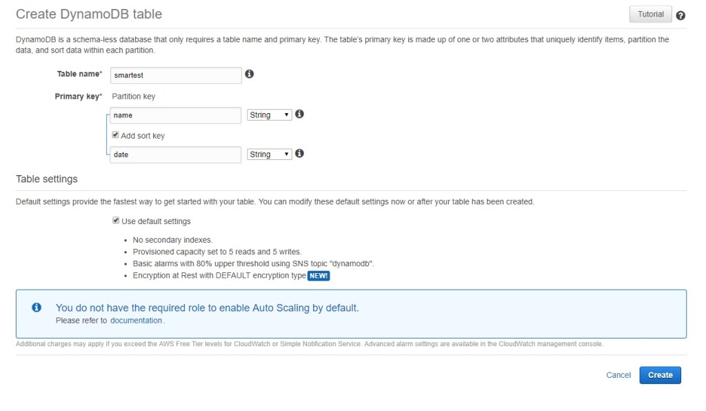
Tables

Like traditional SQL databases, DynamoDB uses tables and they support relationships to other tables. This could be one-to-one, one-to-many and many-to-many. Though no normalization rules apply here, it is still a good idea to break data into multiple tables for benefits such as:

• DynamoDB tables have size limits, by breaking into multiple tables we get away from these limits
• DynamoDB charges by record size change, having tables with smaller number of fields is cost savings
• Can create more indexes on each of the tables

1 to 1 relationships are implemented using a common Id field from both tables, much like foreign keys in traditional databases. Just keep track of the key mappings between tables.

1 to many relationships are implemented using a Partition Key and the Sort Key

Many to many relationships are implemented using GSI or LSI keys

Composite keys are combination of multiple keys.

Partition Keys / Sort Keys / Composite Keys

NoSQL is loosely structured in that each item in a table still requires a key. This is known as the partition key and it uniquely identifies an item(s). Note that a partition key is not the same as a primary key where there cannot be repeating primary keys. The partition key (or shard key) can have multiple items and is really what determines how the items are to be sharded, or partitioned. Since items of the the same partition key are sharded together, it improves the read/write time for those items and really helps the overall database scale.

We can add an additional key called the sort key. In combination with the partition key, these keys create what is known as the composite key. The sort is used to organize the partitioned items so that complex queries could be run against those items. The sort key can be used for queries like ‘begins with’, ‘between’, ‘contains’, ‘>’, ‘<‘, etc.

Indexing – Local Secondary Index (LSI)

Secondary Indexes may be defined to help organize the partitions. As shown below, the data is stored on disk with first the Keys Only (partition, sort, LSI), then with a projected attribute and finally the full original table.

• Select a different sort order for a partition key (basically its a secondary key)
• Similar to sort keys but values can be duplicated
• Limited by size of single partition
• Note that DynamoDB limits – can only have 5 LSI or GSI per table.

Global Secondary Index (GSI)

This is a completed different aggregation storage method. It uses a separate partition key and optional sort key. In the background, DynamoDB is creating separate tables using the GSIs. See the example below. GSI are powerful when we want to have different queries against the same dataset. The example below shows how the initial base table has a partition key on A1. To access the same data set efficiently with the other columns (A2 – A5) we create GSI per those columns. Note how DynamoDB is creating multiple tables for each of those GSI. The GSI tables are created with an eventual consistency model where each write to the base table initiates a write to the GSI tables. Note that DynamoDB can only have 5 LSI or GSI per table.

Data Types Supported 

• String
• Integer
• Binary (Base64 encoding string)
• Boolean
• Null
• List
• Sets
  • Strings
  • Numbers
  • Objects

The maximum item size in DynamoDB is 400 KB, which includes both attribute name binary length (UTF-8 length) and attribute value lengths (again binary length).

The format is JSON. The following are key types:

• Simple Key
  • Partition Key (unique, usually a hash)
• Composite Key
  • Partition Key
  • Sort Key

Example of Simple Key is a Users table where the UserId is a simple partition key. Example of a Composite Key table is a blog post table where it contains a UserId field as the partition key but also a timestamp field as the sort key. Together they create the composite key.

Aggregations

NoSQL is focused on reducing compute power, not storage. Therefore it is possible and welcomed to have repeating data. We can take advantage of this when needing to provide aggregation methods. Since a DynamoDB table itself cannot do functions such as “count” or “sum”, we would track these records on another table. These tables can be managed by triggers through AWS Lambda.

Also – assume we have an initial table that has fields id, first name and last name. On this table id is the main partition key. But lets say we have another data access requirement for getting items based on first name and on last name. Again, since storage is not priority, we could simply replicate the initial table into 2 more tables, each one having the first or last name as it’s main partition key.

Scans

A method of querying data. This uses an arbitrary search expressions. Scans are convenient but are much slower and expensive to execute. Scans should be used as last resort.

Object Persistence Interface

Maps a DynamoDB table to an object. The object will have certain annotations such as the partition key and attribute name definitions.

Conditional Updates and Optimistic Locking

This resolves write conflicts when multiple requests access the same data. In traditional SQL databases we would use transactions (or Unit of Work Pattern) to deal with this. For NoSQL databases we use a condition that checks for an attribute and executes the update only when the condition is met. This can be done programmatically, outside of DynamoDB. For example, one way to do this is to have a version field that gets incremented every time it is updated.

In the example code below, this can be seen in the Item object as.

@DynamoDBVersionAttribute
privateLongversion;

    public Item put(Item item) {
        mapper.save(item, DynamoDBMapperConfig
                .builder()
                .withSaveBehavior(DynamoDBMapperConfig.SaveBehavior.CLOBBER)
                .build());

        return item;
    }

Finally the code below shows the condition check on the update class so that both updates can happen simultaneously.

    private static void updateDescription(ItemDao itemDao, Item item) {
        while (true) {
            try {
                item.setDescription("Retina display");
                itemDao.update(item);
                break;
            } catch (ConditionalCheckFailedException ex) {
                item = itemDao.get(item.getId());
            }
        }
    }

Transactions

The above section showed how to do locks programmatically using conditions and optimistic locks. We could also programmatically implement transactions to make our database mimic SQL db transaction feature. AWS provides a library for this called TransactionManager. When calling this DynamoDB will store the record in a separate shadow table before saving it to the original table.

Replications

DynamoDB does three (3) AZ (availability zones) replication. By default, every write will not be acknowledged until at least two nodes (or AZ) have completed the write. On read it will get the item that exists on at least 2 nodes. This way, data in dynamoDB guarantees replication on write and read.

Design Patterns

Many best practices and common design patterns can be found here on AWS DynamoDB site:

https://docs.aws.amazon.com/amazondynamodb/latest/developerguide/best-practices.html

It is important to select a partition key that is unique but also easily distributed. The thing to note is that the partition key is what determines the shard/partition/bucket the data will fall into. If we selected a partition key that is too unique, like an auto-incrementing counter, it would distribute our data too sparsely. On the other hand if we selected a key where the access is heavy on certain value(s), it could cause a hot partition. This can be seen when we do a heat map analysis. The following shows a single partition having more transactions than others – indicating that partition key is more heavily focused.

A best practice is to focus on how the data will be accessed and partition the keys as such.

Many to Many Relationships

When dealing with many-to-many relationships a common best practice is to use the adjacency list design pattern. This is where we create multiple tables with different partition keys. This is particularly useful when dealing with nested data and wanting to have the initial base table contain the nested values.

DynamoDB Encryption at Rest

Amazon DynamoDB offers fully managed encryption at rest. This is provided by default as of 12.2017. All data at rest is encrypted using encryption keys stored in AWS Key Management Service (AWS KMS). This functionality helps reduce the operational burden and complexity involved in protecting sensitive data. With encryption at rest, you can build security-sensitive applications that meet strict encryption compliance and regulatory requirements.

DynamoDB encryption at rest provides an additional layer of data protection by securing your data in the encrypted table, including its primary key, local and global secondary indexes, streams, global tables, backups, and DynamoDB Accelerator (DAX) clusters whenever the data is stored in durable media. Organizational policies, industry or government regulations, and compliance requirements often require the use of encryption at rest to increase the data security of your applications.

Encryption at rest integrates with AWS KMS for managing the encryption key that is used to encrypt your tables. If we dont want to use KMS, we can use the default type where it is owned and stored in DynamoDB.

• AWS owned CMK – Default encryption type. The key is owned by DynamoDB (no additional charge).
• AWS managed CMK – The key is stored in your account and is managed by AWS KMS (AWS KMS charges apply).

DynamoDB API

When configuring DynamoDB we need to specify the RCU and WCU (Read/Write requests). If these settings are lower than actual, it can handle the overload with a burst capacity, but this is limited. Eventually this will result in an error so it is important to set the RCU/WCU up front correctly.

The APIs use HTTP methods. Example:

POST / HTTP/1.1
Host: dynamodb.us-east2.amazonaws.com;
...
X-Amz-Date: 20160811T123
X-Amz-Target: DynamoDB_20160101.GetItem
{
 "TableName": "mytable",
 "Key": {
  "UserId": {"N" : "1"},
  "Timestamp": {"N": "2018010112345" {
 }
}

The available API methods are:

• Tables
  • CreateTable
  • UpdateTable
  • DescribeTable
  • DeleteTable
  • ListTables
• Item*
  • PutItem
  • GetITem
  • UpdateItem
  • DeleteItem
• Items (Batch)
  • BatchGetItem – multiple items by key
  • BatchWriteItem – 25 items per put or delete
• Query – using composite keys
• Scan – full table scan
• Others
  • DescribeTimeToLive, UPdateTimeToLive
  • TagResource, UntagResource, ListTagsOfResource
  • DescribeLimits

*The Item calls can contain conditions. This is useful for doing this like updating a counter.

Sample Code using DynamoDB API

The following are some sample code (java) in defining a table programmatically using the aws.dynamodb library. This will be migrated into DynamoDB programmatically shown later below. Note the annotations that make these objects mapped to the DynamoDB table.

import com.amazonaws.services.dynamodbv2.datamodeling.*;

@DynamoDBTable(tableName = "Items")
public class Item {

    @DynamoDBAutoGeneratedKey
    @DynamoDBHashKey
    private String id;

    @DynamoDBAttribute
    private String name;

    @DynamoDBAttribute
    private String description;

    @DynamoDBAttribute
    private int totalRating;

    @DynamoDBAttribute
    private int totalComments;

    @DynamoDBVersionAttribute
    private Long version;

    public String getId() {
        return id;
    }
...

The following is a sample code that uses the DynamoDBMapper’s CreateTableRequest to create the tables. Note how we are also setting up the GSI and LSI here programmatically.

import com.amazonaws.services.dynamodbv2.AmazonDynamoDB;
import com.amazonaws.services.dynamodbv2.datamodeling.DynamoDBMapper;
import com.amazonaws.services.dynamodbv2.model.*;
import com.amazonaws.services.dynamodbv2.transactions.TransactionManager;
public class Utils {

    public static void createTables(AmazonDynamoDB dynamoDB) {
        DynamoDBMapper dynamoDBMapper = new DynamoDBMapper(dynamoDB);

        createTable(Item.class, dynamoDBMapper, dynamoDB);
    }

    private static void createTable(Class<?> itemClass, DynamoDBMapper dynamoDBMapper, AmazonDynamoDB dynamoDB) {
        CreateTableRequest createTableRequest = dynamoDBMapper.generateCreateTableRequest(itemClass);
        createTableRequest.withProvisionedThroughput(new ProvisionedThroughput(1L, 1L));

        if (createTableRequest.getGlobalSecondaryIndexes() != null)
            for (GlobalSecondaryIndex gsi : createTableRequest.getGlobalSecondaryIndexes()) {
                gsi.withProvisionedThroughput(new ProvisionedThroughput(1L, 1L));
                gsi.withProjection(new Projection().withProjectionType("ALL"));
            }

        if (createTableRequest.getLocalSecondaryIndexes() != null)
            for (LocalSecondaryIndex lsi : createTableRequest.getLocalSecondaryIndexes()) {
                lsi.withProjection(new Projection().withProjectionType("ALL"));
            }

        if (!tableExists(dynamoDB, createTableRequest))
            dynamoDB.createTable(createTableRequest);

        waitForTableCreated(createTableRequest.getTableName(), dynamoDB);
        System.out.println("Created table for: " + itemClass.getCanonicalName());

    }
...

Below is some sample data access code (java) to interact with the newly created table.

import com.amazonaws.services.dynamodbv2.AmazonDynamoDB;
import com.amazonaws.services.dynamodbv2.datamodeling.DynamoDBMapper;
import com.amazonaws.services.dynamodbv2.datamodeling.DynamoDBMapperConfig;
import com.amazonaws.services.dynamodbv2.datamodeling.DynamoDBScanExpression;

import java.util.List;

public class ItemDao {

    private final DynamoDBMapper mapper;

    public ItemDao(AmazonDynamoDB dynamoDb) {
        this.mapper = new DynamoDBMapper(dynamoDb);
    }

    public Item put(Item item) {
        mapper.save(item, DynamoDBMapperConfig
                .builder()
                .withSaveBehavior(DynamoDBMapperConfig.SaveBehavior.CLOBBER)
                .build());

        return item;
    }

    public Item get(String id) {
        return mapper.load(Item.class, id);
    }

    public void update(Item item) {
        mapper.save(item);
    }

    public void delete(String id) {
        Item item = new Item();
        item.setId(id);

        mapper.delete(item);
    }

    public List getAll() {
        return mapper.scan(Item.class, new DynamoDBScanExpression());
    }
}

DynamoDB Streams

This is a feature used for real-time updates, such as cross-region replication or real-time processing. This does not support scans or transactions.

Another popular use case for using DynamoDB Streams is to update CloudSearch.

DynamoDB Streams can be implemented using lower level API code provided through the AWS developer libraries, or using AWS Kinesis library. Note in the diagram above we’re using a Lambda function for updating CloudSearch. This is triggered by DynamoDB (configured in the Lambda console under the triggers tab). The Lambda function must have the correct role to access CloudSearch and DynamoDB access.

Data Search using AWS CloudSearch

For doing text searches we can utilize the CloudSearch service, which is basically a managed search service running on top of Apache Solr. It will import data from DynamoDB and run the actual search. Another benefit is that CloudSearch has ranking ability and therefore rank our search results. Note that there is a limitation in that only up to 5MB of data can be searched at once from DynamoDB.

DAX – DynamoDB Accelerator

certain use cases that require response times in microseconds. For these use cases, DynamoDB Accelerator (DAX) delivers fast response times for accessing eventually consistent data.

DAX is a DynamoDB-compatible caching service that enables you to benefit from fast in-memory performance for demanding applications. DAX addresses three core scenarios:

• As an in-memory cache, DAX reduces the response times of eventually-consistent read workloads by an order of magnitude, from single-digit milliseconds to microseconds.
• DAX reduces operational and application complexity by providing a managed service that is API-compatible with Amazon DynamoDB, and thus requires only minimal functional changes to use with an existing application.
• For read-heavy or bursty workloads, DAX provides increased throughput and potential operational cost savings by reducing the need to over-provision read capacity units. This is especially beneficial for applications that require repeated reads for individual keys.

DAX supports server-side encryption. With encryption at rest, the data persisted by DAX on disk will be encrypted. DAX writes data to disk as part of propagating changes from the primary node to read replicas. For more information, see DAX Encryption at Rest.

AWS EMR and Apache Hadoop

Whereas DynamoDB is the NoSQL database responsible for the read and write of data, Hadoop is a tool/framework we use to perform data analysis on that data. The NoSQL database provides fast read/writes with the horizontal scalability (and dynamic changing of data formats/schemas) so that can get data into our storage. Hadoop then takes that dataset and by using MapReduce, is able to compute the data quickly over large distributions. NoSQL and Hadoop work together to provide the ‘big data’ solution.

The Hadoop stack includes various software such as the HDFS storage system and the MapReduce query system that sits on top of it. There various tools AWS provides to create a Hadoop cluster. AWS’s EMR service runs Hadoop projects. It is an elastic service and supports many tools such as Spark and Flink.

Apache Hive is an ad hoc data analysis tool for distributed data like those in HDFS / Hadoop. It supports SQL-92 specification. Basically it converts the SQL into MapReduce jobs. Note that Hive is not a database and should not be treated like one because it has high latencies. The queries can be run directly from DynamoDB or copies of the data either on S3 or HDFS. This would all be done inside AWS EMR.

AWS CloudWatch

This is AWS monitoring service that collects and tracks metrics on various other services in AWS such as DynamoDB. We can set alarms which trigger emails or other actions, such as auto-scaling. Some of the metrics CloudWatch can monitor on DynamoDB are:

• Throughput – Consumed Read/Write Capacity Units
• Data Returned – number records returned, size of records
• Failures
• Other

AWS CloudTrail

CloudTrail stores metadata of all requests inside of AWS. It is a service that provides Audit trail, information for security analysis, or troubleshooting errors. Such metadata are:

• Who made request
• API called
• Timestamp
• Call parameters

All this information can be stored inside DyanmoDB or S3. This information is also forwarded to CloudWatch so that we can monitor it and set alarms.

References

RDS API User Guide
https://docs.aws.amazon.com/AmazonRDS/latest/UserGuide/Welcome.html

AWS DynamoDB Deep Dive (pluralsight)
Ivan Mushketyk; 2017
https://app.pluralsight.com/player?course=aws-dynamodb-deep-dive

DynamoDB Encryption at Rest
https://docs.aws.amazon.com/amazondynamodb/latest/developerguide/EncryptionAtRest.html
https://docs.aws.amazon.com/amazondynamodb/latest/developerguide/encryption.usagenotes.html

DAX
https://docs.aws.amazon.com/amazondynamodb/latest/developerguide/DAX.concepts.html

Hadoop and NoSQL
https://mapr.com/blog/hadoop-vs-nosql-whiteboard-walkthrough/

AWS Conference (Initial release)
https://www.youtube.com/watch?v=E9gYor8W2oY

SQL to NoSQL Best Practicies
https://www.youtube.com/watch?v=RLxWobyd2Tc

Running through DynamoDB Sample
https://www.youtube.com/watch?v=qcIzpEHyHwo